Evaluation¶

Given a dataset of items where a user has implicitly or explicitly interacted with (via ratings, purchases, downloads, previews, etc.), the idea is to split the dataset in two—usually disjunct—sets. The training and test datasets.

The evaluation package implements several metrics such as: predictive accuracy (Mean Absolute Error, Root Mean Square Error), decision based (Precision, Recall, F–measure), and rank based metrics (Spearman’s $\rho$ , Kendall– $\tau$ , and Mean Reciprocal Rank)

For a complete list of available metrics to evaluate recommender systems see [http://research.microsoft.com/pubs/115396/EvaluationMetrics.TR.pdf]

Given a test set $\mathcal{T}$ of user-item pairs $(u, i)$ with ratings $r_{ui}$ , the system generates predicted ratings $\hat{r}_{ui}$ .

Prediction-based metrics¶

Predictive metrics aim at comparing the predicted values against the actual values. The result is the average over the deviations.

Mean Absolute Error¶

[http://en.wikipedia.org/wiki/Mean_absolute_error]

Mean Absolute Error (MAE) measures the deviation between the predicted and the real value:

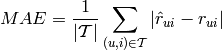
$MAE = \frac{1}{|\mathcal{T}|}\sum_{(u,i) \in \mathcal{T}} \left| \hat{r}_{ui} - r_{ui} \right|$

where $\hat{r}_{ui}$ is the predicted value of user $u$ for item $i$ , and $r_{ui}$ is the true value (ground truth).

Examples¶

from recsys.evaluation.prediction import MAE

mae = MAE()
mae.compute(4.0, 3.2) #returns 0.8

from recsys.evaluation.prediction import MAE

DATA_PRED = [(3, 2.3), (1, 0.9), (5, 4.9), (2, 0.9), (3, 1.5)]
mae = MAE(DATA_PRED)
mae.compute() #returns 0.7

from recsys.evaluation.prediction import MAE

GROUND_TRUTH = [3.0, 1.0, 5.0, 2.0, 3.0]
TEST = [2.3, 0.9, 4.9, 0.9, 1.5]
mae = MAE()
mae.load_ground_truth(GROUND_TRUTH)
mae.load_test(TEST)
mae.compute() #returns 0.7

Root Mean Squared Error¶

[http://en.wikipedia.org/wiki/Root_mean_square_deviation]

Mean Squared Error (MSE) is also used to compare the predicted value with the real value a user has assigned to an item. The difference between MAE and MSE is that MSE heavily penalise large errors.

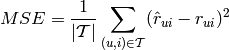
$MSE = \frac{1}{|\mathcal{T}|}\sum_{(u,i) \in \mathcal{T}} (\hat{r}_{ui} - r_{ui})^2$

Root Mean Squared Error (RMSE) equals to the square root of the MSE value.

$RMSE = \sqrt{MSE}$

Examples¶

from recsys.evaluation.prediction import RMSE

rmse = RMSE()
rmse.compute(4.0, 3.2) #returns 0.8

from recsys.evaluation.prediction import RMSE

DATA_PRED = [(3, 2.3), (1, 0.9), (5, 4.9), (2, 0.9), (3, 1.5)]
rmse = RMSE(DATA_PRED)
rmse.compute() #returns 0.891067

Decision-based metrics¶

Decision-based metrics evaluates the top-N recommendations for a user. Uusally recommendations are a ranked list of items, ordered by decreasing relevance. Yet, the decision-based metrics do not take into account the position -or rank- of the item in the result list).

There are four different cases to take into account:

True positive (TP). The system recommends an item the user is interested in.
False positive (FP). The system recommends an item the user is not interested in.
True negative (TN). The system does not recommend an item the user is not interested in.
False negative (FN). The system does not recommend an item the user is interested in.

	Relevant	Not relevant
Recommended	TP	FP
Not recommended	FN	TN

Precision (P) and recall (R) are obtained from the 2x2 contingency table (or confusion matrix) shown in the previous Table.

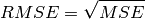
Precision¶

[http://en.wikipedia.org/wiki/Precision_and_recall]

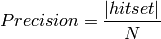
Precision measures the fraction of relevant items over the recommended ones.

$Precision=\frac{TP}{TP+FP}$

Precision can also be evaluated at a given cut-off rank, considering only the top–n recommendations. This measure is called precision–at–n or P@n.

When evaluating the top–n results of a recommender system, it is quite common to use this measure:

$Precision=\frac{|hit set|}{N}$

where $|hit set|=|test \cap topN|$ .

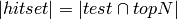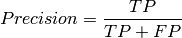
Recall¶

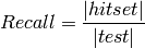
Recall measures the coverage of the recommended items, and is defined as:

$Recall=\frac{TP}{TP+FN}$

Again, when evaluating the top–N results of a recommender system, one can use this measure:

$Recall=\frac{|hit set|}{|test|}$

F-measure¶

[http://en.wikipedia.org/wiki/F1_score]

F–measure combines P and R results, using the weighted harmonic mean. The general formula (for a non-negative real $beta$ value) is:

$F_\beta = \frac{(1 + \beta^2) \cdot (\mathrm{precision} \cdot \mathrm{recall})}{(\beta^2 \cdot \mathrm{precision} + \mathrm{recall})}$

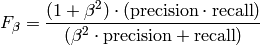
Two common F–measures are $F_{1}$ and $F_{2}$ . In $F_{1}$ recall and precision are evenly weighted, whilst $F_{2}$ weights recall twice as much as precision.

Example¶

from recsys.evaluation.decision import PrecisionRecallF1

TEST_DECISION = ['classical', 'invented', 'baroque', 'instrumental']
GT_DECISION = ['classical', 'instrumental', 'piano', 'baroque']
decision = PrecisionRecallF1()
decision.load(GT_DECISION, TEST_DECISION)
decision.compute() # returns (0.75, 0.75, 0.75)
                   # P = 3/4 (there's the 'invented' result)
                   # R = 3/4 ('piano' is missing)

The main drawback of the decision–based metrics is that do not take into account the ranking of the recommended items. Thus, an item at top–1 has the same relevance as an item at top–20. To avoid this limitation, we can use rank–based metrics.

Rank-based metrics¶

Spearman’s rho¶

[http://en.wikipedia.org/wiki/Spearman’s_rank_correlation_coefficient]

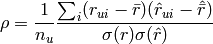
Spearman’s $\rho$ computes the rank–based Pearson correlation of two ranked lists. It compares the predicted list with the user preferences (e.g. the ground truth data), and it is defined as:

$\rho = \frac{1}{n_u} \frac{\sum_i( r_{ui} - \bar{r}) ( \hat{r}_{ui} - \hat{\bar{r}} ) }{\sigma(r) \sigma(\hat{r})}$

Examples¶

Using explicit ranking information:

from recsys.evaluation.ranking import SpearmanRho

TEST_RANKING = [('classical', 25.0), ('piano', 75.0), ('baroque', 50.0), ('instrumental', 25.0)]
GT_RANKING = [('classical', 50.0), ('piano', 100.0), ('baroque', 25.0), ('instrumental', 25.0)]
spearman = SpearmanRho()
spearman.load(GT_RANKING, TEST_RANKING)
spearman.compute() #returns 0.5

Rank-based correlation for ratings:

from recsys.evaluation.ranking import SpearmanRho

DATA_PRED = [(3, 2.3), (1, 0.9), (5, 4.9), (2, 0.9), (3, 1.5)]
spearman = SpearmanRho(DATA_PRED)
spearman.compute() #returns 0.947368

Kendall–tau¶

[http://en.wikipedia.org/wiki/Kendall_tau_rank_correlation_coefficient]

Kendall– $\tau$ also compares the recommended ( $topN$ ) list with the user’s preferred list of items. Kendall– $\tau$ rank correlation coefficient is defined as:

$\tau = \frac{C^+ - C^-}{\frac{1}{2}{N(N-1)}}$

where $C^+$ is the number of concordant pairs, and $C^-$ is the number of discordant pairs in the data set.

Examples¶

Using explicit ranking information:

from recsys.evaluation.ranking import KendallTau

TEST_RANKING = [('classical', 25.0), ('piano', 75.0), ('baroque', 50.0), ('instrumental', 25.0)]
GT_RANKING = [('classical', 50.0), ('piano', 100.0), ('baroque', 25.0), ('instrumental', 25.0)]
kendall = KendallTau()
kendall.load(GT_RANKING, TEST_RANKING)
kendall.compute() #returns 0.4

Rank-based correlation for ratings:

from recsys.evaluation.ranking import KendallTau

DATA_PRED = [(3, 2.3), (1, 0.9), (5, 4.9), (2, 0.9), (3, 1.5)]
kendall = KendallTau(DATA_PRED)
kendall.compute() #returns 0.888889

Mean reciprocal Rank¶

[http://en.wikipedia.org/wiki/Mean_reciprocal_rank]

Mean Reciprocal Rank (MRR) is defined as:

$\text{MRR} = \frac{1}{|Q|} \sum_{i=1}^{Q} \frac{1}{\text{rank}_i}$

Recommendations that occur earlier in the top–n list are weighted higher than those that occur later in the list.

Example¶

Computing reciprocal rank ( $RR=\frac{1}{\text{rank}_i}$ ) for one query:

from recsys.evaluation.ranking import ReciprocalRank

GT_DECISION = ['classical', 'instrumental', 'piano', 'baroque']
QUERY = 'instrumental'
rr = ReciprocalRank()
rr.compute(GT_DECISION, QUERY) #returns 0.5 (1/2): found at position (rank) 2

Mean reciprocal rank for a list of queries $Q$ :

from random import shuffle
from recsys.evaluation.ranking import MeanReciprocalRank

TEST_DECISION = ['classical', 'invented', 'baroque', 'instrumental']
GT_DECISION = ['classical', 'instrumental', 'piano', 'baroque']
mrr = MeanReciprocalRank()
for QUERY in TEST_DECISION:
    shuffle(GT_DECISION) #Just to "generate" a different GT each time...
    mrr.load(GT_DECISION, QUERY)
mrr.compute() #in my case, returned 0.45832

Mean Average Precision¶

[http://en.wikipedia.org/wiki/Mean_average_precision]

Mean Average Precision ( $MAP$ ) is defined as:

$\text{MAP} = \frac{\sum_{q=1}^Q AP(q)}{Q}$

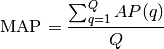
where $Q$ is the number of queries, and $Average Precision$ (AP) [http://en.wikipedia.org/wiki/Mean_average_precision#Average_precision] equals:

$\text{AP} = \frac{\sum_{k=1}^n (P(k) \times rel(k))}{\mbox{number of relevant documents}}$

where $P(k)$ is Precision at top-k, and $rel(k)$ is an indicator function equaling 1 if the item at rank is a relevant document, and zero otherwise.

Recommendations that occur earlier in the top–n list are weighted higher than those that occur later in the list.

Example¶

Computing average Precision ( $AP$ ) for one query, $q$ :

from recsys.evaluation.ranking import AveragePrecision

ap = AveragePrecision()

GT = [1,2,3,4,5]
q = [1,3,5]
ap.load(GT, q)
ap.compute() # returns 1.0

GT = [1,2,3,4,5]
q = [99,3,5]
ap.load(GT, q)
ap.compute() # returns 0.5833335

Mean Average Precision for a list of retrieved results $Q$ :

from recsys.evaluation.ranking import MeanAveragePrecision

GT = [1,2,3,4,5]
Q = [[1,3,5], [99,3,5], [3,99,1]]
Map = MeanAveragePrecision()
for q in Q:
    Map.load(GT, q)
Map.compute() # returns 0.805556

Evaluation¶

Prediction-based metrics¶

Mean Absolute Error¶

Examples¶

Root Mean Squared Error¶

Examples¶

Decision-based metrics¶

Precision¶

Recall¶

F-measure¶

Example¶

Rank-based metrics¶

Spearman’s rho¶

Examples¶

Kendall–tau¶

Examples¶

Mean reciprocal Rank¶

Example¶

Mean Average Precision¶

Example¶

Table Of Contents

Previous topic

Next topic

This Page

Navigation

Evaluation¶

Prediction-based metrics¶

Mean Absolute Error¶

Examples¶

Root Mean Squared Error¶

Examples¶

Decision-based metrics¶

Precision¶

Recall¶

F-measure¶

Example¶

Rank-based metrics¶

Spearman’s rho¶

Examples¶

Kendall–tau¶

Examples¶

Mean reciprocal Rank¶

Example¶

Mean Average Precision¶

Example¶

Table Of Contents

Previous topic

Next topic

This Page

Quick search

Navigation